
Introduction
This topic will be oriented toward techniques which can be used to interpret nondestructive testing, NDT, data from the Falling Weight Deflectometer, FWD. There are all kinds of NDT data which can be collected on or about pavements but concentration is placed on measured surface deflections. This article is separated into three broad themes: (1) an introduction, (2) indices for project analysis, and (3) fundamentals of backcalculation. The introduction will start with an overview of some of the deflection basic parameters that have been used in the past; although, some of the NDT equipment noted is rarely used today (such as the Dynaflect). This is followed by a discussion of some easy to use models to predict layer moduli that were developed by the University of Washington for the Washington State DOT (WSDOT). A short discussion on AASHTO developed models follows along with some of the work done in South Africa and companies such as the Shell Oil Co. The second theme will cover basic parameters which can be quite useful in analyzing existing pavement structures. The last theme focuses on the basics associated with backcalculation of layer moduli. These basics do not rely on specific software but do largely involve layered elastic analysis.
Deflection Basin Parameters
Over the years numerous techniques have been developed to analyze deflection data from various kinds of pavement deflection equipment. A fairly complete summary of deflection basin parameters was provided by Horak at the Sixth International Conference Structural Design of Asphalt Pavement [Horak, 1987[1]] and is shown in Table 1.
Table 1. Summary of Deflection Basin Parameters [modified from Horak, 1987[1]
| Parameter | Formula | Measuring Device |
|---|---|---|
| Maximum deflection | D0 | Benkelman Beam, Lacroux deflectometer, FWD |
| Radius of curvature | R = r2/2 D0(D0/Dr – 1); r = 5″ | Curvaturemeter |
| Spreadability | S = + D1 + D2 + D3/5100/D0; D1 … D3 spaced 12″ apart | Dynaflect |
| Area | A = 6[1 + 2 (D1/D0) + 2 (D2/ D0) + D3/D0); with sensors located at 0, 1, 2, 3 ft | FWD |
| Shape factors | F1 = (D0 -D2) / D1 and F2 = (D1 -D3) / D2 | FWD |
| Surface curvature index | SCI = D0 – Dr, where r = 12″ or r = 20″ | Benkelman Beam, Road Rater, FWD |
| Base curvature index | BCI = D24″ – D36″ | Road Rater |
| Base damage index | BDI = D12″ – D24″ | Road Rater |
| Deflection ratio | Qr = Dr/D0, where Dr ≈ D0/2 | FWD |
| Bending index | BI = D/a, where a = Deflection basin | Benkelman Beam |
| Slope of deflection | SD = tan-1 (D0 – Dr )/r where r = 24 in. | Benkelman Beam |
All of these parameters tend to focus on four major areas:
- Plate or center load deflection which represents the total defection of the pavement. This was obviously the first deflection parameter which came with the Benkelman Beam. It has been used for many years as the primary input for several overlay design procedures.
- The slope or deflection differences close to the load such as Radius of Curvature (R), Shape Factor (F1), and Surface Curvature Index (SCI). These parameters tend to reflect the relative stiffness of the bound or upper regions of the pavement section.
- The slope or deflection differences in the middle of the basin about 11.8 in. (300 mm) to 35.4 in. (900 mm) from the center of the load. These parameters tend to reflect the relative stiffness of the base or lower regions of the pavement section.
- The deflections toward the end of the basin. Deflections in this region relate quite well to the stiffness of the subgrade below the pavement surfacing.
The subsequent parameters to be presented were developed to provide a means of obtaining the resilient modulus values of the surfacing layers more easily or quickly than full backcalculation. In general, the success of these regression equations to predict the resilient modulus of the surfacing layers has been limited. There is a clear consensus, however, that the deflections measured beyond the primary effects of the load stress bulb relate quite well to the resilient modulus of the subgrade.
WSDOT Equations
Several researchers have developed regression equations to predict the subgrade modulus, ESG, from plate load and deflections measured at distances from about 24 in. (600 mm) to 48 in. (1200 mm) from the center of the plate load. Newcomb developed such regression equations to predict ESG as part of an overall effort to develop a mechanistic empirical overlay design procedure for WSDOT [Newcombe, 1986 [2]]. For two layer cases, the subgrade modulus, can be estimated from:
| ESG = -466 + 0.00762 (P/D3), where 3 = 3 feet from middle of the load plate (Eq. 1) |
| ESG = -198 + 0.00577 (P/D4), where 4 = 4 feet from middle of the load plate (Eq. 2) |
| ESG = -371 + 0.00671 (2P/(D3 + D4)), (Eq. 3) |
and for three layer cases:
| ESG = -530 + 0.00877 (P/D3), (Eq. 4 |
| ESG = -111 + 0.00577 (P/D4), (Eq. 5) |
| ESG = -346 + 0.00676 (2P/(D3 + D4)) (Eq. 6) |
The R2 ≈ 99% for all equations and the sample sizes were 180 (two layer case) and 1,620 (three layer case).
These equations were developed from generated data (ELSYM5) with the following levels of input data: (Tables 2 and 3)
Table 2: Two Layer Cases
| Load, P, lb (kN) | Surface Thickness, hAC, in. (mm) | Surface Modulus, EAC, psi (MPa) | Subgrade Modulus, ESG, psi (MPa) |
|---|---|---|---|
| 5,000 (22) | 2 (50) | 2,000,000 (13800) | 50,000 (345) |
| 10,000 (44) | 6 (150) | 500,000 (3450) | 30,000 (207) |
| 15,000 (67) | 12 (300) | 100,000 (690) | 10,000 (69) |
| 18 (450) | 5,000 (35) | ||
| 2,500 (17) |
Table 3: Three Layer Cases
| Load, P, lb (kN) | Surface Thickness, hAC, in. (mm) | Base Thickness, hB, in (mm) | Surface Modulus, EAC, psi (MPa) | Base Modulus, EB, psi (MPa) | Subgrade Modulus, ESG, psi (MPa) |
|---|---|---|---|---|---|
| 5,000 (22) | 2 (50) | 4 (100) | 2,000,000 (13800) | 100,000 (690) | 50,000 (345) |
| 10,000 (44) | 6 (150) | 10 (250) | 500,000 (3450) | 50,000 (345) | 30,000 (207) |
| 15,000 (67) | 12 (300) | 18 (450) | 100,000 (690) | 30,000 (207) | 10,000 (69) |
| 10,000 (69) | 5,000 (35) | ||||
| 2,500 (17) |
(assumed that load applied on a 11.8 in. (300 mm) diameter load plate)
From this generated data (no rigid base), regression equations were also developed for estimating the surface modulus (AC) for a two layer case (for example a “full-depth” pavement):
| log EAC = -0.53740 – 0.95144 log10 ESG -1.2118(hAC)0.33 + 1.78046 log10 PA1/D02) (Eq. 7) |
where R2 = 0.83
For a three layer case, equations were developed for both EAC and EB as follows:
If both EAC and EB unknown:
| log EAC = -4.13464 + 0.25726 (5.9/hAC) + 0.92874(5.9/hB)0.5 – 0.69727 (hAC/hB)0.5 – 0.96687 log10 ESG + 1.88298 log10 (PA1/D02) (Eq. 8) |
where R2 = 0.78.
| log EB = 0.50634 + 0.03474 (5.9/hAC) + 0.12541(5.9/hB)0.5 – 0.09416 (hAC/hB)0.5 + 0.51386 log ESG + 0.25424 log10 (PA1/D02) (Eq. 9) |
where R2 = 0.70.
The following variables were used in the equations shown above:
P = applied load (lbs) on a 11.8 in. (300 mm) plate,
hAC = surface course thickness (in.),
hB = base course thickness (in.),
EAC = surface course modulus (psi),
EB = base course modulus (psi),
ESG = subgrade modulus (psi),
D0 = deflection under center of applied load (in.),
D0.67 = deflection at 8 in. (0.67 ft) from center of applied load (in.),
D1 = deflection at 1 ft from center of applied load (in.),
D2= deflection at 2 ft from center of applied load (in.),
D3 = deflection at 3 ft from center of applied load (in.),
D4 = deflection at 4 ft from center of applied load (in.), and
A1 = approximate area under deflection basin out to 3 ft = 2 + D0.67) + (D0.67 + D1) + 3(D1 + D2) + 3(D2 + D3) = 4D0 + 6D0.67 + 8D1 + 12D2 + 6D3
AASHTO Equations
Witczak presented a similar regression equation in Part III of the 1986 AASHTO Guide for Design of Pavement Structures [AASHTO, 1986[3]]. That equation is in the form:
| ESG = (P)(Sf)/(Dr)(r) (Eq. 10) |
where
P = plate load (lb),
Sf = subgrade modulus prediction factor,
= 0.2686 for µ = 0.50
= 0.2792 for µ = 0.45
= 0.2892 for µ = 0.40
= 0.2874 for µ = 0.35
= 0.2969 for µ = 0.30
Dr = pavement surface deflection measured at r distance, from the load, and
r = distance from the load to Dr (in.).
Using an Sf value of 0.2892 where the Poisson’s ratio is 0.40, the equation reduces to the following equations for deflections measured at 2 ft (610 mm), 3 ft (914 mm), and 4 ft. (1,219 mm).
| ESG = 0.01205(P/D2) (Eq. 11) |
| ESG = 0.00803(P/D3) (Eq. 12) |
| ESG = 0.00603(P/D4) (Eq. 13) |
In the AASHTO Guide, detailed procedures are provided to insure that the deflections used to determine ESG are outside the pressure bulb from the test load. To most accurately represent the subgrade stiffness; however, the deflections closest to the load without being directly effected by the pressure bulb should be used. Stiff underlying layers will have the greatest effect on deflections furthermost from the test load. For example in cases where total surfacing depths are around 11.8 in. (300 mm), deflections taken around 23.6 in. (600 mm) should be used to determine ESG.
A NCHRP study [Darter et al., 1991[4]] was used to revise Part III of the AASHTO Pavement Guide [AASHTO, 1986[3]], it is recommended that the following equation be used to solve for subgrade modulus:
| MR = P(1 – µ2)/(π)(Dr)(r) (Eq. 14) |
where
MR = backcalculated subgrade resilient modulus (psi),
P = applied load (lbs),
Dr = pavement surface deflection a distance r from the center of the load plate (inches), and
r = distance from center of load plate to Dr (inches).
Using a Poisson’s ratio of 0.40, Equation 14 reduces to
| MR = 0.01114 (P/D2) (Eq. 15) |
| MR = 0.00743 (P/D3) (Eq. 16) |
| MR = 0.00557 (P/D4) (Eq. 17) |
for sensor spacings of 2 ft (610 mm), 3 ft (914 mm), and 4 ft (1219 mm). If a Poisson’s ratio of 0.45 is used instead for the same sensor spacings, the equations become:
| MR = 0.01058(P/D2) (Eq. 18) |
| MR = 0.00705 (P/D3) (Eq. 19) |
| MR = 0.00529 (P/D4) (Eq. 20) |
Darter et al. [1991[4]] recommends that the deflection used for subgrade modulus determination should be taken at a distance at least 0.7 times r/ae where r is the radial distance to the deflection sensor and ae is the radial dimension of the applied stress bulb at the subgrade “surface.” The ae dimension can be determined from the following:
ae =  [4]] recommends that the deflection used for subgrade modulus determination should be taken at a distance at least 0.7 times r/ae where r is the radial distance to the deflection sensor and ae is the radial dimension of the applied stress bulb at the subgrade "surface." The ae dimension can be determined from the following:" width="150" height="48" srcset="https://pavementinteractive.org/wp-content/uploads/2010/04/RadiusOfStressBulb-e1317744778387-180x58.jpg 180w, https://pavementinteractive.org/wp-content/uploads/2010/04/RadiusOfStressBulb-e1317744778387-300x97.jpg 300w, https://pavementinteractive.org/wp-content/uploads/2010/04/RadiusOfStressBulb-e1317744778387.jpg 526w" sizes="(max-width: 150px) 100vw, 150px" />
where
ae = radius of stress bulb at the subgrade-pavement interface,
a = NDT load plate radius (inches),
D = total thickness of pavement layers (inches)
EP = effective pavement modulus (psi), and
MR = backcalculated subgrade resilient modulus.
For “thin” pavements (such as Section A, Figure 3), ae ≈ 15 in.; “medium” to “thick” pavements (Sections B and C, Figure 3), ae ≈ 26 to 33 in. Thus, the minimum r is usually 24 to 36 in. (recall r > 0.7 (ae)).
South African Equations
A similar relation between deflections taken at 2000 mm (78.7 in.) was shown by Horak [1987][1]:
| log10 ESG = 9,727 – 0.989 log10 δ2000 |
where
ESG = subgrade elastic modulus (Pa), (same as ESG), and
δ2000 = deflection at a distance of 2000 mm from the (point) of loading (µm).
Additional Modulus Estimates
Subgrade Soils
- Table 4 is used to show typical subgrade moduli as listed by Chou et al. [1989[5]].
- CBR Correlation- A classic correlation that has been widely used is:
| ESG (psi) = 1,500 (CBR) |
or
| ESG (MPa) = 10 (CBR) |
where
CBR = California Bearing Ratio
Note: Limited to fine-grained soils with a CBR of 10 or less.
Table 4. Typical Values of Subgrade Moduli [after Chou et al., 1989[5]
| Climate Condition | ||||
| Dry | Wet – No Freeze | Wet - Freeze | ||
| Frozen | Unfrozen | |||
| Material | psi (MPa) | psi (MPa) | psi (MPa) | psi (MPa) |
| Clay | 15,000 (103) | 6,000 (41) | 6,000 (41) | 50,000 (345) |
| Silt | 15,000 (103) | 10,000 (69) | 5,000 (34) | 50,000 (345) |
| Silty or Clayey Sand | 20,000 (138) | 10,000 (69) | 5,000 (34) | 50,000 (345) |
| Sand | 25,000 (172) | 25,000 (172) | 25,000 (172) | 50,000 (345) |
| Silty or Clayey Gravel | 40,000 (276) | 30,000 (207) | 20,000 (138) | 50,000 (345) |
| Gravel | 50,000 (345) | 50,000 (345) | 40,000 (276) | 50,000 (345) |
Granular Materials Shell Method [Chou et al., 1989 [5]; Smith and Witczak, 1981 [6]]
The granular base modulus is a function of the subgrade modulus and base course thickness.
| EB = 0.2(25.4h2)0.45ESG |
where
EB = base modulus (psi),
h2 = base thickness (in.)
ESG = subgrade modulus (psi)
Example
If
ESG = 15,000 psi and the base thickness = 10 in., then
| EB = 0.2(25.4 (10))0.45(15,000) ≈ 36,000 psi (250 MPa) |
Stabilized Base Materials
From Chou et al. [22] [5]:
- Asphalt stabilized materials: use information available for asphalt concrete.
- Lime-stabilized materials: a modulus range of 100,000 to 1,000,000 psi (690 to 6,895 MPa) is suggested.
- Cement stabilized materials: a range of 300,000 to 4,000,000 psi (2,070 to 27,600 MPa) is suggested.
Asphalt Concrete
From Chou et al. [1989[5]]:
- Absolute minimum and maximum values for AC are 50,000 to 2,000,000 psi (345 to 13,790 MPa).
- To estimate the lowest and highest AC moduli, use expected high and low temperatures along with the Asphalt Institute equation [ASTM, 1984[7]] which is of the form:
| | E* | = f (P200, f, Vv, η70˚F, T, Pac) |
where
| E* | = dynamic modulus (stiffness of asphalt concrete),
P200 = percent aggregate passing No. 200 sieve,
f = frequency of loading,
Vv = percent air voids,
η70˚F = original absolute viscosity used in mix at 70F (21.1C)
T = temperature, and
Pac = asphalt content, by weight of mix.
Chou et al. [1989[5]] use default values of
P200 = 6%
f = 25 Hz
Vv = 7%
η70˚F = 106 poises
Pac = 5%
Indices For Project Analysis
Introduction
Over the years it has found that the use of selected indices and algorithms provide a “good picture” of the relative conditions found throughout a project. This picture is very useful in performing backcalculation and may at times be used by themselves on projects with large variations in surfacing layers.
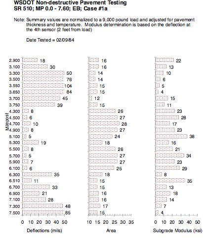
WSDOT is currently using deflections measured at the center of the test load combined with Area values and ESG computed from deflections measured at 24 in. (610 mm) presented in a linear plot to provide a visual picture of the conditions found along the length of any project (as illustrated in Figure 1).
Area Parameter
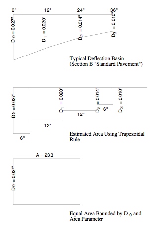
The Area value represents the normalized area of a slice taken through any deflection basin between the center of the test load and 3 ft (914 mm). By normalized, it is meant that the area of the slice is divided by the deflection measured at the center of the test load, D0. Thus the Area value is the length of one side of a rectangle where the other side of the rectangle is D0. The actual area of the rectangle is equal to the area of the slice of the deflection basin between 0 and 3 ft (914 mm).
The original Area equation is:
| A = 6(D0 + 2D1 + 2D2 + D3)/D0 |
where
D0 = surface deflection at center of test load,
D1 = surface deflection at 1 ft (305 mm),
D2 = surface deflection at 2 ft (610 mm), and
D3 = surface deflection at 3 ft (914 mm).
The approximate metric equivalent of this equation is:
| A = 150(D0 + 2D300 + 2D600 + D900)/D0 |
where
D0 = deflection at center of test load,
D300 = deflection at 300 mm,
D600 = deflection at 600 mm, and
D900 = deflection at 900 mm.
Figure 2 shows the development of the normalized area for the Area value using the Trapezoidal Rule to estimate area under a curve.
The basic Trapezoidal Rule is:
| K = h (1/2y0 + y1 + y2 + 1/2y3) |
where
K = any planar area,
y0 = initial chord,
y1, y2 = immediate chords,
y3 = last chord, and
h = common distance between chords.
Thus, to estimate the area of a deflected basin using D0, D1, D2, and D3, and h = 6 in., then:
| K = 6 (D0 + 2D1 + 2D2 + D3) |
Further, normalize by dividing by D0:
| Area = (6/D0)*(D0 + 2D1 + 2D2 + D3) |
or
| Area = 6 (1 +2D1/D0 + 2D2/D0 + D3/D0) |
Thus, since we normalized by D0, the Area Parameter’s unit of measure is inches (or mm) not in2 or mm2 as one might expect.
The maximum value for Area is 36.0 (915 mm) and occurs when all four deflection measurements are equal (not likely to occur) as follows:
If, D0 = D1 = D2 = D3
Then, Area = 6(1 + 2 + 2 + 1) = 36.0 in.
For all four deflection measurements to be equal (or nearly equal) would indicate an extremely stiff pavement system (like portland cement concrete slabs or thick, full-depth asphalt concrete.)
The minimum Area value should be no less than 11.1 in. (280 mm).
This value can be calculated for a one-layer system which is analogous to testing (or deflecting) the top of the subgrade (i.e., no pavement structure). Using appropriate equations, the ratios of
| D1/D0 , D2/D0, D3/D0 |
always result in 0.26, 0.125, and 0.083, respectively. Putting these ratios in the Area equation results in:
| Area = 6(1+ 2(0.26) + 2(0.125) + 0.083) = 11.1 in. |
Further, this value of Area suggests that the elastic moduli of any pavement system would all be equal (e.g., E1 = E2 = E3 = …). This is highly unlikely for actual, in-service pavement structures. Low area values suggest that the pavement structure is not much different from the underlying subgrade material (this is not always a bad thing if the subgrade is extremely stiff — which doesn’t occur very often).
Typical Area values were computed for pavement Sections A, B, and C (Figure 3) and are shown in Table 5 (along with the calculated surface deflections (D0, D1, D2, D3)). Table 6 provides a general guide in the use of Area values obtained from FWD pavement surface deflections. For Figure 3, the initial layer moduli are HMA = 500,000 psi, crushed stone base = 25,000 psi, and fine-grained subgrade = 7,500 psi.
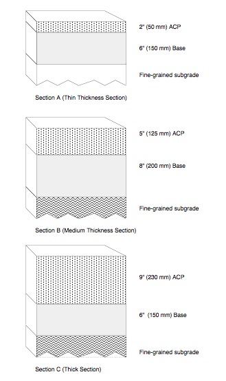
Table 5: Estimates of Area from Pavement Sections – Cases A, B, and C
| Pavement Cases | Pavement Surface Deflections, inches | Area | ||||
| D0 | D1 | D2 | D3 | in. | (mm) | |
| Standard Pavement (HMA @ 500,000 psi, base course @ 25,000 psi, and subgrade @ 7,500 psi) | ||||||
| Section A (thin) | 0.048 | 0.026 | 0.014 | 0.009 | 17.1 | (434) |
| Section B (med) | 0.027 | 0.020 | 0.014 | 0.010 | 23.3 | (592) |
| Section C (thick) | 0.018 | 0.015 | 0.012 | 0.009 | 27.0 | (686) |
| Stabilize Subgrade (upper 6 in. of subgrade increased from 7,500 to 50,000 psi) | ||||||
| Section A (thin) | 0.036 | 0.020 | 0.013 | 0.009 | 18.5 | (470) |
| Section B (med) | 0.023 | 0.017 | 0.012 | 0.009 | 23.5 | (597) |
| Section C (thick) | 0.016 | 0.013 | 0.011 | 0.009 | 27.4 | (696) |
| Asphalt Treated Base (increase base course modulus from 25,000 to 500,000 psi) | ||||||
| Section A (thin) | 0.021 | 0.018 | 0.013 | 0.010 | 26.6 | (676) |
| Section B (med) | 0.014 | 0.012 | 0.010 | 0.009 | 28.7 | (729) |
| Section C (thick) | 0.012 | 0.011 | 0.009 | 0.008 | 30.0 | (762) |
| Moisture Sensitivity (decrease HMA modulus from 500,000 to 200,000 psi) | ||||||
| Section A (thin) | 0.053 | 0.026 | 0.014 | 0.009 | 16.1 | (409) |
| Section B (med) | 0.033 | 0.022 | 0.014 | 0.009 | 20.7 | (526) |
| Section C (thick) | 0.024 | 0.018 | 0.013 | 0.010 | 24.0 | (610) |
Table 6: Trends of D0 and Area Values
| FWD Based Parameter | Generalized Conclusions* | |
| Area | Maximum Surface Deflection (D0) | |
| Low | Low | Weak structure, strong subgrade |
| Low | High | Weak structure, weak subgrade |
| High | Low | Strong structure, strong subgrade |
| High | High | Strong structure, weak subgrade |
Naturally, exceptions can occur.
Table 7: Typical Area Values
| Pavement | Area | |
| in. | (mm) | |
| PCCP | 24-33 | (610-840) |
| “Sound” PCC* | 29-32 | (740-810) |
| BST flexible pavement (relatively thin structure) | 15-17 | (380-430) |
| Thick ACP (≥ 4.2 in. HMA) | 21-30 | (530-760) |
| Weak BST | 12-15 | (300-380) |
| Thin ACP (< 4.2 in. HMA) | 16-21 | (410-530) |
from 1993 AASHTO Guide, p. III-117
Fundamentals of Backcalculation
Introduction
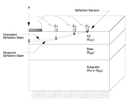
A method which has received extensive development work is the “backcalculation” method. This is essentially a mechanistic evaluation of pavement surface deflection basins generated by various pavement deflection devices. Backcalculation is one where measured and calculated surface deflection basins are matched (to within some tolerable error) and the associated layer moduli required to achieve that match are determined. The backcalculation process is usually iterative and normally done with software. An illustration of the backcalculation process is shown in Figure 4.
Typical Flowchart
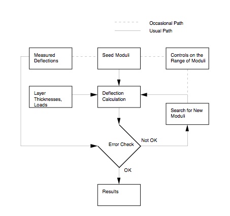
A basic flowchart which represents the fundamental elements in all known backcalculation programs is shown as Figure 5. This flowchart was patterned after one shown by Lytton (1989[8]). Briefly, these elements include:
- Measured deflections – Includes the measured pavement surface deflections and associated distances from the load.
- Layer thicknesses and loads – Includes all layer thicknesses and load levels for a specific test location.
- Seed moduli – The seed moduli are the initial moduli used in the computer program to calculate surface deflections. These moduli are usually estimated from user experience or various equations.
- Deflection calculation – Layered elastic computer programs are generally used to calculate a deflection basin.
- Error check – This element simply compares the measured and calculated basins. There are various error measures which can be used to make such comparisons (more on this in a subsequent paragraph in this section).
- Search for new moduli – Various methods have been employed within the various backcalculation programs to converge on a set of layer moduli which produces an acceptable error between the measured and calculated deflection basins.
- Controls on the range of moduli – In some of the backcalculation programs, a range (minimum and maximum) of moduli are selected or calculated to prevent program convergence to unreasonable moduli levels (could be too high or low).
Measure of Convergence
Measure of Deflection Basin Convergence
In backcalculating layer moduli, the measure of how well the calculated deflection basin matches (or converges to) the measured deflection basin was previously described as the “error check.” This is also referred to as the “goodness of fit” or “convergence error.”
The primary measure of convergence will be Root Mean Square (RMS) or Root Mean Square Error (RMSE) and is used in the EVERCALC program. Both terms are taken to be the same.
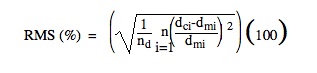
where
RMS = root mean square error,
dci = calculated pavement surface deflection at sensor i,
dmi = measured pavement surface deflection at sensor i, and
nd = number of deflection sensors used in the backcalculation process.
Example RMS Calculation
| nd | Deflections (mils) | |
| Measured | Calculated | |
| 1 (0″) | 5.07 | 4.90 |
| 2 (8″) | 4.32 | 3.94 |
| 3 (12″) | 3.67 | 3.50 |
| 4 (18″) | 2.99 | 3.06 |
| 5 (24″) | 2.40 | 2.62 |
| 6 (36″) | 1.69 | 1.86 |
| 7 (60″) | 1.01 | 0.95 |
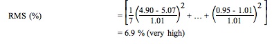
Generally an adequate range of RMS is 1 to 2 percent.
Depth of Stiff Layer
Research provided at least two approaches for estimating the depth to stiff layer [Rohde and Scullion, 1990[9]; Hossain and Zaniewski, 1991[10]]. The approach used by Rohde and Scullion [1990[9]] will be summarized below. There are two reasons for this selection: (1) initial verification of the validity of the approach is documented, and (2) the approach is used in MODULUS and EVERCALC — backcalculation programs widely used in the U.S.
(a) Basic Assumptions and Description
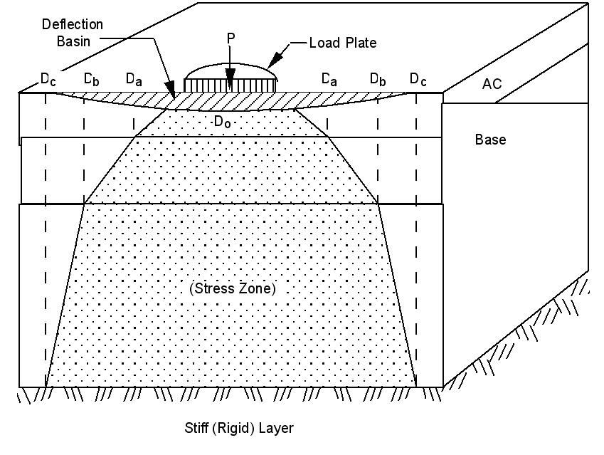
A fundamental assumption is that the measured pavement surface deflection is a result of deformation of the various materials in the applied stress zone; therefore, the measured surface deflection at any distance from the load plate is the direct result of the deflection below a specific depth in the pavement structure (which is determined by the stress zone). This is to say that only that portion of the pavement structure which is stressed contributes to the measured surface deflections. Further, no surface deflection will occur beyond the offset (measured from the load plate) which corresponds to the intercept of the applied stress zone and the stiff layer (the stiff layer modulus being 100 times larger than the subgrade modulus). Thus, the method for estimating the depth to stiff layer assumes that the depth at which zero deflection occurs (presumably due to a stiff layer) is related to the offset at which a zero surface deflection occurs. This is illustrated in Figure 6 where the surface deflection Dc is zero.
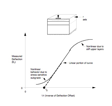
An estimate of the depth at which zero deflection occurs can be obtained from a plot of measured surface deflections and the inverse of the corresponding offsets (1/r). This is illustrated in Figure 7. The middle portion of the plot is linear with either end curved due to nonlinearities associated with the upper layers and the subgrade. The zero surface deflection is estimated by extending the linear portion of the D vs. 1/r plot to a D = 0, the 1/r intercept being designated as r0. Due to various pavement section-specific factors, the depth to stiff layer cannot be directly estimated from r0 — additional factors must be considered. To do this, regression equations were developed based on BISAR computer program generated data for the following factors and associated values:
Load = P = 9000 lbs (40 kN) (only load level considered)
Moduli ratios:
| E1/ESG = 10, 30, 100 |
| E2/ESG = 0.3, 1.0, 3.0, 10.0 |
| Erigid/ESG = 100 |
Thickness levels:
| T1 = 1, 3, 5, and 10 in. (25, 75, 125, 250 mm) |
| T2 = 6, 10, and 15 in. (150, 250, 375 mm) |
| B = 5, 10, 15, 20, 25, 30, and 50 ft (1.5, 3.0, 4.5, 6.0, 7.5, 9.0, 15.0 m) |
where
Ei = elastic modulus of layer i,
Ti = thickness of layer i,
B = depth of the rigid (stiff) layer measured from the pavement surface (ft).
The resulting regression equations follow in (b).
(b) Regression Equations
Four separate equations were developed for various HMA layer thicknesses. The dependent variable is 1/B and the independent variables are r0 (and powers of r0) and various deflection basin shape factors such as SCI, BCI, and BDI.
(i) HMA less than 2 in. (50 mm) thick
| 1/B = 0.0362 – 0.3242 (r0) + 10.2717 (r02) – 23.6609 (r03) – 0.0037 (BCI) |
R2 = 0.98
(ii) HMA 2 to 4 in. (50 to 100 mm) thick
| 1/B = 0.0065 + 0.1652 (r0) + 5.4290 (r02) – 11.0026 (r03) – 0.0004 (BDI) |
R2 = 0.98
(iii) HMA 4 to 6 in. (100 to 150 mm) thick
| 1/B = 0.0413 + 0.9929 (r0) – 0.0012 (SCI) + 0.0063 (BDI) – 0.0778 (BCI) |
R2 = 0.94
(iv) HMA greater than 6 in. (150 mm) thick
1/B = 0.0409 + 0.5669 (r0) + 3.0137 (r02) + 0.0033 (BDI) – 0.0665 log (BCI)
R2 = 0.97
where
r0 = 1/r intercept (extrapolation of the steepest section of the D vs. 1/r plot) in units of 1/ft
SCI = D0 – D12″ (D0 – D305mm), Surface Curvature Index,
BDI = D12″ – D24″ (D305 – D610mm), Base Damage Index,
BCI = D24″ – D36″ (D610 – D914mm), Base Curvature Index,
Di = surface deflections (mils) normalized to a 9,000 lb (40 kN) load at an offset i in feet.
(c) Example
Use typical deflection data to estimate B (depth to stiff layer). The drillers log suggests a stiff layer might be encountered at a depth of 198 in. (5.0 m).
(i) First, calculate normalized deflections (9,000 lb (40 kN) basis).
Table 8. Normalized Deflections
| Load Level | Deflections (mils) | ||||||
| D0 | D8 | D12 | D18 | D24 | D36 | D60 | |
| 9,512 lb | 5.07 | 4.32 | 3.67 | 2.99 | 2.40 | 1.69 | 1.01 |
| 9,000 lb (normalized) | 4.76 | 4.04 | 3.44 | 2.80 | 2.26 | 1.59 | 0.95 |
| 6,534 lb | 3.28 | 2.69 | 2.33 | 1.88 | 1.56 | 1.09 | 0.68 |
(ii) Second, estimate r0. Plot Dr vs. 1/r (refer to Figure 7) :
Table 9. Table of Values Dr vs. 1/r
| Dr (mils) | r | 1/r(1/ft) |
|---|---|---|
| 4.76 | 0″ | — |
| 4.04 | 8″ | 1.50 |
| 3.44 | 12″ | 1.00 |
| 2.80 | 18″ | 0.67 |
| 2.26 | 24″ | 0.50 |
| 1.59 | 36″ | 0.33 |
| 0.95 | 60″ | 0.20 |
where all Dr normalized to 9,000 lb (40 kN)
(iii) Third, use regression equation in (b)(iv) (for HMA = 7.65 in. (194 mm)) to calculate B:
| 1/B = 0.0409 + 0.5669 (r0) + 3.0137 (r02) + 0.0033 (BDI) – 0.0665 log (BCI) |
where
r0 = 1/r intercept (refer to Figure 8)
≈ 0 (used steepest part of deflection basin which is for Sensors at 36 and 60 inches)
BDI = D12″ – D24″ = 3.44 – 2.26 = 1.18 mils
BCI = D24″ – D36″ = 2.26 – 1.59 = 0.67 mils
| 1/B = 0.0409 + 0.5669 (0) + 3.0137 (02) + 0.0033 (1.18) – 0.0665 log (0.67) |
= 0.0564
| 1/B = 10.0564 = 17.7 feet (213 inches or 5.4 m) |
This values agrees fairly well with “expected” stiff layer conditions at 16.5 feet (5.0 m) as indicated by the drillers log even though the 1/r value equaled zero.

Example of Depth to Stiff Layer Estimates – Road Z-675 (Sweden)
(a) Overview:
This road located in south central Sweden is used to illustrate calculated and measured depths to stiff layers (the stiff layer apparently being rock for the specific road).
(b) Measurement of Measured Depth:
The depth to stiff layer was measured using borings (steel drill) and a mechanical hammer. The hammer was used to drive the drill to “refusal.” Thus, the measured depths could be to bedrock, a large stone, or hard till (glacially deposited material). Further, the measured depths were obtained independently of the FWD deflection data (time difference of several years).
(c) Deflection Measurements:
A KUAB 50 FWD was used to obtain the deflection basins. All basins were obtained within ± 5 m (16 ft) of a specific borehole. The deflection sensor locations were set at 0, 200, 300, 450, 600, 900, and 1200 mm (0, 7.9, 11.8, 17.7, 23.6, 35.4, and 47.2 in.) from the center of the load plate.
(d) Calculations:
The equations described in Section 3.3.4 were used to calculate the depth to stiff layer. Since the process requires a 9000 lb (40 kN) load and 1 ft (305 mm) deflection sensor spacings, the measured deflections were adjusted linearly according to the ratio of the actual load to a 9000 lb (40 kN) load.
(e) Results:
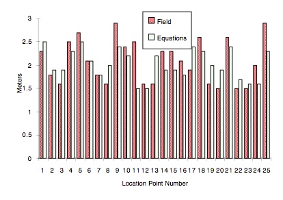
The results of this comparison are shown in Figure 9. Given all the uncertainties concerning the measured depths, the agreement is quite good.
Verification of Backcalculation Results
There have been and, undoubtedly, will be a number of attempts to verify that backcalculated layer moduli are “reasonable.” One way to do this is to compare measured, in-situ strains to calculated (theoretical) strains based on layered elastic analyses.
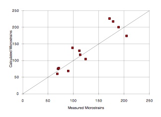
Two studies have done this. The first study summarized (Winters, 1993[11]) was conducted at the PACCAR Technical Center located at Mt. Vernon, Washington. Horizontal strains were measured on asphalt concrete instrumented cores (inserted into the original asphalt concrete surface material). The HMA layer was approximately 5.5 in. thick over a 13.0 in. thick base course. The WSDOT FWD was used to apply a known load to induce the strain response (measured strain). The calculated strains were determined by use of the EVERCALC program (which used FWD deflection basins to backcalculate layer moduli which, in turn, were used to calculate the corresponding strains.)
Figures 10 and 11 show the measured and calculated strains in the two horizontal directions at the bottom of the AC layer (longitudinal and transverse). This specific testing was conducted during February 1993. In general, the agreement is good.

The second study was reported by Lenngren [1990[12]]. That work was conducted for RST Sweden and used backcalculated layer moduli (from a modified version of the EVERCALC program) to estimate strains at the bottom of two thicknesses of HMA (3.1 and 5.9 in. thick). The pavement structures were located in Finland. Tables 10 and 11 are used as summaries. The backcalculated strains are generally within ± 5 percent of the measured strains.
Table 10. Backcalculated and Measured Tensile Strains – 3.1 in. (80 mm) HMA Section (1990)
| Time of Day (a.m. or p.m.) | Tensile Strain Bottom of HMA (x 10-6) | ||
| Backcalculated* | Measured | % Difference | |
| a.m. | 119 | 123 | -3 |
| a.m. | 119 | 122 | -2 |
| a.m. | 74 | 64.9 | +14 |
| a.m. | 60 | 64.7 | -8 |
| p.m. | 284 | 292 | -3 |
| p.m. | 284 | 283 | ~0 |
| p.m. | 167 | 159 | +5 |
| p.m. | 167 | 158 | +6 |
| p.m. | 87 | 84.8 | +2 |
| p.m. | 81 | 84.2 | -4 |
- Backcalculation process used sensors @ D0, D300, D600, D900, and D1200
Table 11. Backcalculated and Measured Tensile Strains —5.9 in. (150 mm) AC Section (1990)
| Time of Day (a.m. or p.m.) | Tensile Strain Bottom of AC (x 10-6) | ||
| Backcalculated* | Measured | % Difference | |
| a.m. | 66 | 69.5 | -6 |
| a.m. | 71 | 69.0 | +3 |
| a.m. | 68 | 68.7 | -1 |
| a.m. | 38 | 34.7 | +9 |
| a.m. | 127 | 130 | -2 |
| a.m. | 119 | 130 | -8 |
| p.m. | 178 | 185 | -4 |
| p.m. | 182 | 183 | -1 |
| p.m. | 104 | 95.9 | +8 |
| p.m. | 51 | 48.0 | +6 |
| p.m. | 56 | 48.5 | +14 |
- ”The Use of Surface Deflection Basin Measurements in the Mechanistic Analysis of Flexible Pavements,” Proceedings, Vol. 1, Sixth International Conference Structural Design of Asphalt Pavements, University of Michigan, Ann Arbor, Michigan, USA, 1987.↵
- Newcomb, D. E., “Development and Evaluation of Regression Methods to Interpret Dynamic Pavement Deflections,” Ph.D. Dissertation, Department of Civil Engineering, University of Washington, Seattle, Washington, 1986.↵
- AASHTO Guide for Design of Pavement Structures, American Association of State Highway and Transportation Officials, Washington, D.C., 1986.↵
- Darter, M.I., Elliott, R.P., and Hall, K.T., “Revision of AASHTO Pavement Overlay Design Procedure,” Project 20-7/39, National Cooperative Highway Research Program, Transportation Research Board, Washington, D.C., September 1991.↵
- Chou, Y. J., Uzan, J., and Lytton, R. L., “Backcalculation of Layer Moduli from Nondestructive Pavement Deflection Data Using the Expert System Approach,” Nondestructive Testing of Pavements and Backcalculation of Moduli , ASTM STP 1026, American Society for Testing and Materials, Philadelphia, 1989, pp. 341 – 354.↵
- Smith. B. E. and Witczak, M. W., “Equivalent Granular Base Moduli: Prediction,” Journal of Transportation Engineering, Vol. 107, TE6, American Society of Civil Engineering, November 1981.↵
- ”Standard Method of Indirect Tension Test for Resilient Modulus of Bituminous Mixtures,” D4123-82, Volume 04.03, American Society for Testing and Materials, Philadelphia, PA, 1984.↵
- Lytton, R.L., “Backcalculation of Pavement Layer Properties,” Nondestructive Testing of Pavements and Backcalculation of Moduli, ASTM STP 1026, American Society for Testing and Materials, Philadelphia, 1989, pp. 7-38.↵
- Rohde, G.T., and Scullion, T., “MODULUS 4.0: Expansion and Validation of the MODULUS Backcalculation System,” Research Report No. 1123-3, Texas Transportation Institute, Texas A&M University System, College Station, Texas, November 1990.↵
- Hossain, A.S.M., and Zaniewski, J.P., “Detection and Determination of Depth of Rigid Bottom in Backcalculation of Layer Moduli from Falling Weight Deflectometer Data,” Transportation Research Record No. 1293, Transportation Research Board, Washington, D.C., 1991.↵
- Mahoney, J.P., Newcomb, D.E., Jackson, N.C., and Pierce, L.M., “Pavement Moduli Backcalculation Shortcourse,” Course Notes, Washington State Department of Transportation (and Other Agencies), September 1991.↵
- ”The PACCAR Pavement Test Section — Instrumentation and Validation,” Master’s thesis, Department of Civil Engineering, University of Washington, Seattle, Washington, March 1993.↵
- ”Relating Bearing Capacity to Pavement Condition,” Ph.D. Dissertation, Royal Institute of Technology, Department of Highway Engineering, Stockholm, Sweden, 1990.↵